2.5. SciPY

last update: May 09, 2024

SciPy is a collection of mathematical algorithms and convenience functions built on the NumPy extension of Python. - scippy doc

In this page, you see examples of scipy functions (differentiation, integration, optimization) to solve problems.

import numpy as np
import matplotlib.pyplot as plt
from scipy import integrate, diff, optimize

from IPython.display import display, Latex

2.5.1. Differentiation

scipy.integrate.solve_ivp

Solve an initial value problem for a system of ODEs.

\[ \frac{dy}{dt} = f(t, y), \quad y(t_0) = y_0 \]

scipy.integrate.solve_ivp(fun, t_span, y0, method='RK45', t_eval=None,\
   dense_output=False, events=None, vectorized=False, args=None, **options)

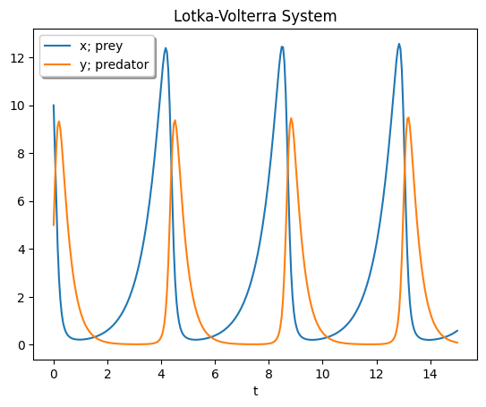
Solve the Lotka-Volterra equations. The Lotka-Volterra equations, also known as the predator-prey equations, are a pair of first-order, non-linear, differential equations frequently used to describe the dynamics of biological systems in which two species interact, one as a predator and the other as prey. They were proposed independently by Alfred J. Lotka in 1925 and Vito Volterra in 1926.

\[ \frac{dx}{dt} = ax - bxy ,\quad \frac{dy}{dt} = -cx + dxy \]

from scipy.integrate import solve_ivp


def lotkavolterra(t, z, a, b, c, d):
    x, y = z
    return [a * x - b * x * y, -c * y + d * x * y]


sol = solve_ivp(lotkavolterra, [0, 15], [10, 5], args=(1.5, 1, 3, 1), dense_output=True)

t = np.linspace(0, 15, 300)
z = sol.sol(t)

plt.plot(t, z.T)
plt.xlabel("t")
plt.legend(["x; prey", "y; predator"], shadow=True)
plt.title("Lotka-Volterra System")
plt.show()

---

2.5.2. Integration

scipy.integrate.quad

Compute a definite integral.

scipy.integrate.quad(func, a, b, args=(), full_output=0, epsabs=1.49e-08, epsrel=1.49e-08,\
   limit=50, points=None, weight=None, wvar=None, wopts=None, maxp1=50, limlst=50)

Return y and abserr.

• y(float): The integral of func from a to b.

• abserr(float): An estimate of the absolute error in the result.

Let’s compute the integral: \( \int_0^4 x^2 dx\)

x2 = lambda x: x**2
ans = integrate.quad(x2, 0, 4)  # numerical result
print("x, y = ", ans)


display(Latex("$$ \int_0^4 x^2 dx = \\frac{x^3}{3} \Big|_0^4 = \\frac{4^3}{3} = 21.3333 $$"))

x, y =  (21.333333333333332, 2.3684757858670003e-13)

\[ \int_0^4 x^2 dx = \frac{x^3}{3} \Big|_0^4 = \frac{4^3}{3} = 21.3333 \]

---

2.5.3. Root finding

scipy.optimize.root_scalar

Find a root of a scalar function.

scipy.optimize.root_scalar(f, args=(), method=None, bracket=None, fprime=None, fprime2=None,\
   x0=None, x1=None, xtol=None, rtol=None, maxiter=None, options=None)

find a root of a scalar function

\[f(x) = x^2 - x -1 \]

from scipy import optimize


def f(x):
    return x**2 - x - 1


sol = optimize.root_scalar(f, bracket=[0, 3])  # numerical result
print("numerical result: ", sol.root)


print("\nanalytical result:")
display(Latex("$$ f(x) = x^2 -x - 1 = 0 \Longleftrightarrow x = \\frac{1 \pm \sqrt{5}}{2} = -0.618034, 1.618034 $$"))

numerical result:  1.618033988749895

analytical result:

\[ f(x) = x^2 -x - 1 = 0 \Longleftrightarrow x = \frac{1 \pm \sqrt{5}}{2} = -0.618034, 1.618034 \]

---

scipy.optimize.root

Find a root of a vector function.

scipy.optimize.root(func, x0, args=(), method='hybr', jac=None, tol=None,
                   callback=None, options=None)

def fun(x):
    return [x[0] + 0.5 * (x[0] - x[1]) ** 3 - 1.0, 0.5 * (x[1] - x[0]) ** 3 + x[1]]


def jac(x):  # Jacbian
    return np.array(
        [
            [1 + 1.5 * (x[0] - x[1]) ** 2, -1.5 * (x[0] - x[1]) ** 2],
            [-1.5 * (x[1] - x[0]) ** 2, 1 + 1.5 * (x[1] - x[0]) ** 2],
        ]
    )


sol = optimize.root(fun, [0, 0], jac=jac, method="hybr")
print('numerical result: ', sol.x)

numerical result:  [0.8411639 0.1588361]

---

scipy.optimize.minimize

Local (multivariate) optimization

scipy.optimize.minimize(fun, x0, args=(), method=None, jac=None, hess=None,\
   hessp=None, bounds=None, constraints=(), tol=None, callback=None, options=None)

find the minimum point of

\[ f(x,y) = (1-x)^2 + 5(y-x^2)^2 \]

from scipy.optimize import minimize

f = lambda x: (1 - x[0]) ** 2 + 5 * (x[1] - x[0] ** 2) ** 2
x0 = [-1, -1]
res = minimize(f, x0, method="CG", options={"disp": True})
print("\nnumerical result: ", res.x)

Optimization terminated successfully.
         Current function value: 0.000000
         Iterations: 12
         Function evaluations: 84
         Gradient evaluations: 28

numerical result:  [0.9999993  0.99999854]

---

scipy.optimize.least_squares

Least-squares

scipy.optimize.least_squares(fun, x0, jac='2-point', bounds=(- inf, inf), method='trf', ftol=1e-08,\
   xtol=1e-08, gtol=1e-08, x_scale=1.0, loss='linear', f_scale=1.0, diff_step=None, tr_solver=None,\
   tr_options={}, jac_sparsity=None, max_nfev=None, verbose=0, args=(), kwargs={})

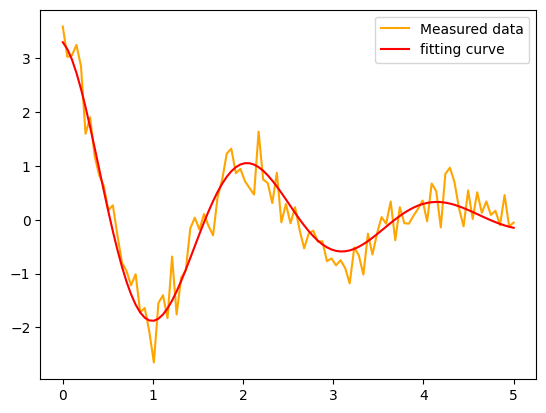
Here, we solve fitting problem.

# Solve a nonlinear least-squares problem with bounds on the variables.
import os
import scipy.optimize as opt

# p: parameters, t: time, y: measured data
fitFunc = lambda p, t: p[0] * np.exp(-p[1] * t) * np.cos(p[2] * t)
errFunc = lambda p, t, y: fitFunc(p, t) - y

np.random.seed(0)
x = np.linspace(0, 5, 100)
y = fitFunc([3, 0.5, 3], x) + np.random.randn(len(x)) / 3

p0 = [1, 1, 1]  # Initial guess for the parameters
(p, success) = opt.leastsq(errFunc, p0, args=(x, y))
print("\nnumerical result: ", p)
print("true value: ", [3, 0.5, 3])
nfit = fitFunc(p, x)

plt.plot(x, y, label="Measured data", color="orange")
plt.plot(x, nfit, label="fitting curve", color="red")
plt.legend()
plt.show()

numerical result:  [3.296355   0.55072818 2.98677005]
true value:  [3, 0.5, 3]